


__crash_absorber_support_area face setwikiffcd2022:start
Indice
Fem Fundamentals and Chassis Design, spring 2022 course
Lecture Notes
Planar beam structure i.p. and o.o.p. loadings
The beam structure centroidal axis lies on a plane, which is also a symmetry plane for the cross-sections.
Symmetric and skew-symmetric loads with respect to such a plane are called in-plane and out-of-plane loads, respectively.
If the superposition of effects holds (e.g., if the structure behaves linearly) each load set only induces an associated subset of the possible components of internal action, see

Symmetric and skew-symm. parts of a general load
A general load is applied to a symmetric structure in a); in b), c) the loads applied on each half structure is treated separately. In d), e) the action on the loaded portion is halved, and symmetrically propagated to the other portion; those symmetric actions are accumulated in the symmetric part of the load f). In g), h) the action on the loaded portion is halved, and skew-symmetrically propagated on the unloaded portion; those skew-symmetric actions are accumulated in the skew-symmetric part of the load i).
Rollbar-like frame
Maxima worksheet v0001, v0002, rollbar_v0002_checkme_insert.wxmxv0003 v0004 v0005 a link rollbar_v0006.wxmx final version 2022
Quarter ladder frame chassis
quarter_ladder_frame_ffcd2022a.wxmx
quarter_ladder_frame_ffcd2022b.wxmx
quarter_ladder_frame_ffcd2022c.wxmx
quarter_ladder_frame_ffcd2022d.wxmx
quarter_ladder_frame_ffcd2022e.wxmx
OTW profile in torsion
profile_in_torsion_v014bis.mud
profile_in_torsion_v016_3d_hole.048.mud
profile_in_torsion_v017b.mud profile_in_torsion_v018b_href.mud profile_in_torsion_v018b_pref.mud profile_in_torsion_v019b_href.mud profile_in_torsion_v019b_pref.mud profile_in_torsion_v020b_href.mud profile_in_torsion_v020b_pref.mud
A Phoney monocoque chassis
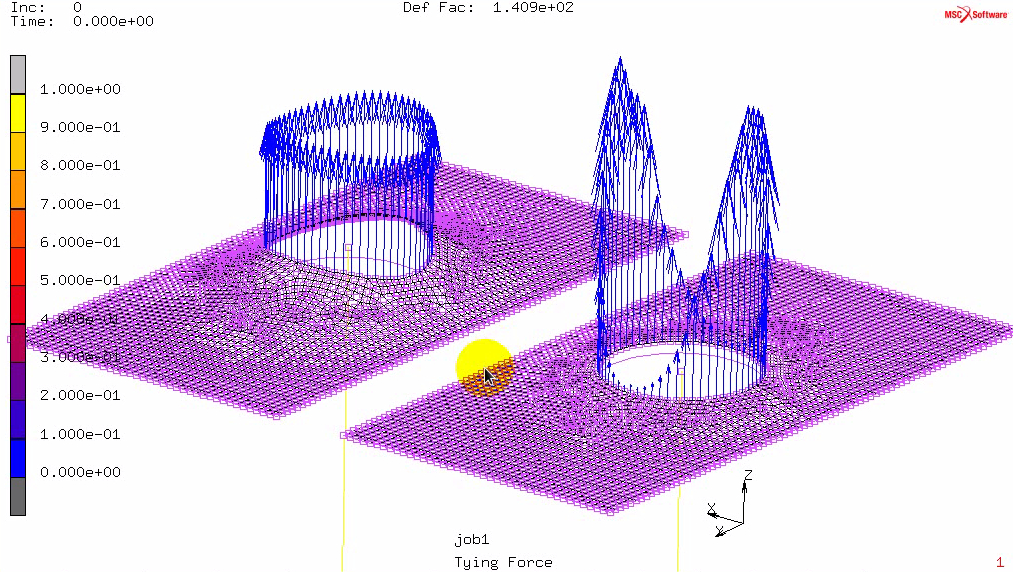
RBE3 connector: kinematics, moment distribution; RBE2 vs. RBE3 demonstrator model, screenshot.
Models: v001, v002, v0031), monocoque_chassis_2022_v003b.mud, v004, v005 2), v203, v203motions, v204, v205, v206, v207.
Properties
Suspension link trusses
Solid circular beam sections, ø12mm, aluminum. Essentially rigid with respect to other chassis structures.
Rear framework
Hollow circular section beam, aluminum.
Main structure: outer diameter ø40mm, wall thickness 1.8mm.
Stiffeners: outer diameter ø30mm, wall thickness 1.2mm.
Composite monocoque
Thicker backbone: 1.8mm aluminum sheet, 25.4mm aluminum honeycomb 3003, density 5.2 lb/ft^3 (hex-3003-td.pdf), 1.8mm aluminum sheet.
Thinner panels: 1.8mm aluminum sheet, 6.75mm same aluminum honeycomb, 1.8mm aluminum sheet.
Frontal shock absorber support plate: provisionally as thinner panels, to be defined based on shock.
Sway (anti-roll) bar
outer diameter ø25mm, wall thickness 2mm, extremely stiff (Super-alloy Z, E=E_steel*1e4, nu=0.3); it may be mechanically isolated at need by deactivating one of the connecting elements to the wheel hub carriers.
Such a “deformable but extremely stiff” linkage modeling should be discouraged in favor of an actual kinematic constraining – i.e. an MPC, since excessive stiffness badly impacts the system matrix condition number (or the integration time step, in the case of explicit dynamic simulations); nonetheless, it allowed for a very straightforward implementation.
Inertial elements modeling
The following spreadsheets are used in defining the equivalent rectangular cuboids for each inertially relevant rigid body: engine, wheel assemblies. The driver inertia is modeled through an 80 kg steel bar spanning roughly from the sternum to the pelvis.
Frontal crash absorber collapse loadcase (inertia relief)
At the element faces belonging to the crash_absorber_bearing_area set (an approx. 155×320 mm area at the front bulkhead), a 25 psi = 0,172 MPa distributed pressure is applied which is due to the honeycomb absorber crushing (see datasheet).
How to set a damped response
Buckling
Sparse material
Videos
Interesting stuff
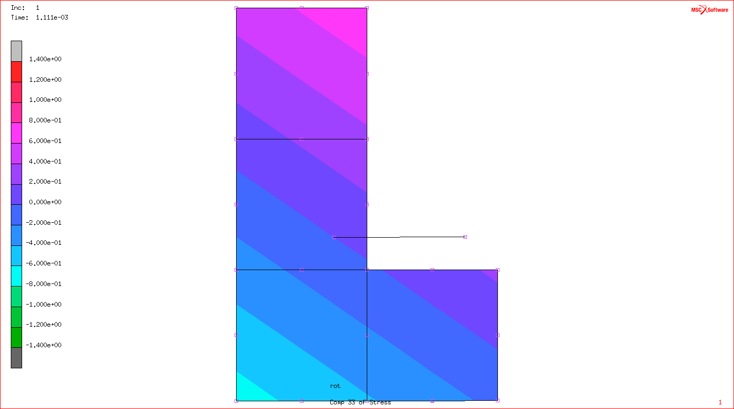
Reference L-shaped cross section, to verify the coupled bending formulas: maxima worksheet, Oxy and G12 oriented MSC.Marc/Mentat linear models. Large rotation, animated hiE lowE models, gif animation.
free_anticlastic_vs_cylindrical_bending.wxmx maxima worksheet for the four point bending test discussion.
Roller bearing questionable modeling
Dynamics related stuff
On the relevance of constraining in dynamic analyses back view side view relevance of (improper) constraints on the dynamic behaviour of a structure. Design is reliable in actual operational conditions (link). Added constraints stiffen up the structure, thus increasing natural frequencies. However, a 0 Hz rigid body mode natural frequency may rise to a finite value due to added positioning constraints; the associate natural mode may be excited in resonance by dynamic loads.
Poor man dynamic response animated view
MSC.Mentat procedure for creating poor man harmonic response animations
MSC.Mentat procedure for creating poor man natural mode animations
Structural damping references
structural_damping_values_jdstevenson.pdf
damping_cross-reference_and_material_properties.pdf
f_orban_damping_of_materials_and_members_in_structures.pdf
tom_irvine_damping_in_bolted_and_welded_joints.pdf
estratto vol. 2, sezione 8 di Soovere, J., and M. L. Drake. Aerospace Structures Technology Damping Design Guide.LOCKHEED-CALIFORNIA CO BURBANK, 1985.
Exercises
Exam turns
1)
with respect to v002, i) I created the truss elements at the front right suspension, ii) I selected also the rotational dofs at the wheel assebly RBE2, and iii) I created the
2)
with respect to v004, i) materials and geometric props are associated to the two truss elements that connect the sway bar to the wheel assemblies, ii) one of those trusses is selectively deactivated in the various jobs, iii) the max along layers eq. von Mises stres is asked as a result
wikiffcd2022/start.txt · Ultima modifica: da ebertocchi