Indice
mentat2013.1 -ogl -glflush
Damped harmonic response
monocoque_chassis_2019_v008.mud
How to set a damped response
In order to include a small degree of structural damping (eg. 1% of the critical value) into a MSC.Marc/Mentat harmonic response calculation, the following steps may be followed:
- enter the menu
MAIN → MATERIAL PROPERTIES → MATERIAL PROPERTIES; - preemptively define a modulating table 1/ω
- menu
TABLES,NEW → 1 INDIPENDENT VARIABLE - define
NAMEasmodulate_stiffmatmult - set Indipendent variable v1
TYPEasfrequency - define table through
FORMULAand type1/pi/v1, i.e. $g(f)=\frac{1}{\pi f}$
- go back to
MAIN → MATERIAL PROPERTIES → MATERIAL PROPERTIESby hittingRETURN; - select the various model materials, and for each of them enter the submenu
STRUCTURAL → DAMPINGand activateDAMPING; - leave alone the
MASS MATRIX MULTIPLIERvalue (0 is ok, otherwise some “structural” damping will be associated to rigid body motions), - define a
STIFFNESS MATRIX MULTIPLIERequal to the desired fraction of the critical value, namely0.01, - set a frequency modulating function, namely TABLE, by hitting the
TABLEbutton on the right of the stiffness matrix multiplier value; - select the just defined
modulate_stiffmatmulttable as the modulating one, hence hitOKandOKagain to return back at the material properties menu - in this way, I defined damping as a function of the $\alpha$ e $\beta$ coefficients introduced by the Rayleigh proportional damping model, with zero $\alpha$ and hence no contribution of the mass matrix. In particular $\zeta = \frac{1}{2}(\frac{\alpha}{2 \pi f}+2 \pi f \beta)$ with $\alpha=0$ and $\beta= 0.01 \cdot g(f)=\frac{0.01}{\pi f}$, from which $\zeta=0.01$ as desired.
- enter the
MAIN → JOBSmenu and create a copy of the undamped harmonic response job by hitting theCOPYtop left button and by setting a new job name; - enter the job
PROPERTIESmenu, and reach theANALYSIS OPTIONSsubmenu; activate theCOMPLEX DAMPINGoptions within the dynamic harmonic section, and then exit withOK - Enter the
JOB RESULTSsubmenu and deactivateStress,Equivalent von Mises stress - substitute them with the AVAILABLE ELEMENT SCALARS
Equivalent Real Harmonic Stress, layersMAX & MINEquivalent Imag Harmonic Stress, layersMAX & MIN- the REAL HARMONIC e IMAG HARMONIC stress resultant equivalents for the beam elements,
DEFAULTlayer, and theBeam Orientatio Vector
- insert from the AVAILABLE ELEMENT TENSORS block
Real Harmonic Stress, layersALLImag Harmonic Stress, layersALL
- run the simulation as usual with
RUN → SUBMIT - open the post file as usual with
OPEN POST FILE (RESULTS MENU) - The deformed shape may be visualized according to a given phase within the oscillation cycle (see also the
DEFORMED SHAPE SETTINGSmenu); in the absence of damping the fase was limited to the 0° and 180° values, cases these that may be represented with the bare variation in sign of the stress and displacement components to be monitored. - Please note that the real component has a 0° phase ($\cos(\omega t)$ modulation) whereas the imaginary component has a 270° phae ($-\sin(\omega t)$ modulation).
- Please also note that in resonance conditions the imaginary component becomes dominant and reaches the peak values, whereas the real component vanishes (resonant response is in fact ~90° out of phase with respect to the real, 0° excitation).
- Lets e.g. collect the displacement in $z$ direction of the node at the center of the excited wheel contact area:
- enter the POSTPROCESSING
RESULTSmenu, with opened t16 result file, and proceed within theHISTORY PLOTsubmenu - define the locations for the response sampling with
SET LOCATIONS, hence click on the desired node[s], and finalize withEND LIST - define the range of the sub-increments to be collected with
INC RANGE, and then entering at the prompt0:1[enter],0:397[enter],1[enter], as the sampling beginning, end and step. - proceed with the definition of collected response diagrams by entering th
ADD CURVESmenu, and thenALL LOCATIONS(a single location has been selected); select theFrequencyglobal variable as the abscissa, and theDisplacement Z Magnitudenodal variable as the ordinate. TheFITscales the axes to contain all the sample points. - By hitting
RETURNI may return to the HISTORY PLOT menu, where the label density may be reducedSHOW IDSfrom '1' to '10'; by entering a '0' value labels are hidden.
- response peaks are now finite (they were theoretically unbounded in the absence of damping), and peaks disappear in correspondence of natural modes that are weakly coupled with the exciting force. In the absence of damping, bounded response at resonance is obtained for strictly uncoupled natural modes only.
Euler column buckling
base model: 400mm_supported_bar.mfd
buckling load evaluation: 400mm_supported_bar.wxmx
model at the end of today's lesson:400mm_supported_barv002.mfd
Flexural-torsional buckling example
simplisupportedprofile_v000.mud
profile made in s235jr steel
thickness:
| thickness | |
|---|---|
| flanges | 4 mm |
| web | 2mm |
| gusset plates at supports | 4 mm |
simply supported at gusset plate - lower flange intersection nodes (support_me node set).
100kN load, uniformly distributed along the intersection line between the upper flange and the web spanning from support to supports (load_me node set).
Please note that in MSC.Marc the supplied point load value is applied to each associated node.
Evaluate the peak equivalent von Mises stress along the structure according to the linear elastic modeling.
Due to the compressive state of the profile web, a check with respect to buckling is also required.
a few notes
Exam like exercises
Tubolar welded T-joint
The mesh elements are created along the midsurface
- Aluminum (E=70000 MPa, nu=0.3, rho=2.7e-9 tonn/mm^3)
- Chord:
- average diameter: 50mm
- wall thickness: 4mm
- Brace:
- average diameter: 40mm
- wall thickness: 2mm
apply a torsional moment passing through the chord s.t. the nominal shear stress according to the beam theory is 1 MPa; evaluate the stress concentration at the joint as the peak equivalent von Mises stress (according to the employed discretization).
Rollbar-like frame structure, o.o.plane transverse load
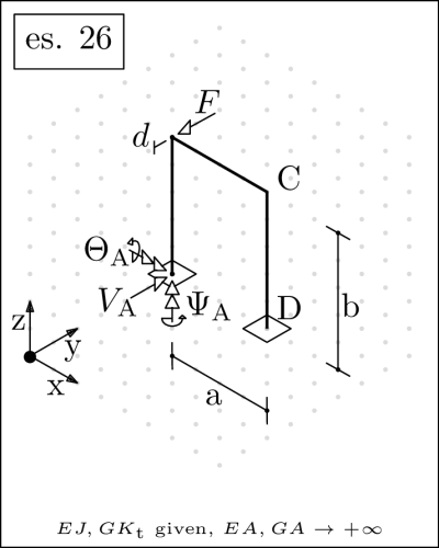
Find the reaction force $V_\mathrm{A}$ and the reaction moments $\Phi_\mathrm{A}, \Psi_\mathrm{A}$ at the base of the directly loaded frame upright member; evaluate then the deflection $d$ at the load application point.
Numerically evaluate the unknown quantities with respect to the following dimensions
dim:	[
            a=800,
            b=1000,
            E=210000,
            G=210000/2/(1+3/10),
            J=(40^4-36^4)*%pi/64,
            Kt=(40^4-36^4)*%pi/32
        ];
Solution: outofplane_loaded_frame_v001.wxmx

